Introduction

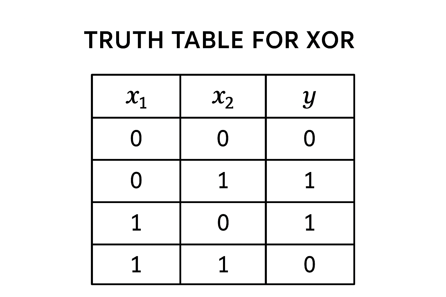
Neural networks have become ubiquitous in modern machine learning, and we'll be exploring how a simple neural network can learn to model the XOR function. The logical XOR function is a nonlinear function that takes two binary inputs, (or commonly boolean inputs of true or false) and produces a binary output. Specifically, the output is 1 if exactly one of the inputs is 1, and 0 otherwise. The truth table for the XOR function is as follows:

Neural Networks

Neural networks are computational models inspired by the structure and function of biological neural networks in the brain. They consist of interconnected nodes, or "neurons," that process and transmit information. An individual neuron has some number of inputs, each with an associated weight, and produces an output based on an activation function. The output of one neuron can be fed as input to other neurons, forming layers of interconnected nodes. Neural networks can learn to perform complex tasks by adjusting the weights of the connections between neurons based on the input data and desired output. Conceptually, we can think of the input as making up the first layer of neurons, the hidden layers as intermediate layers of neurons that process the input, and the output layer as the final layer of neurons that produce the output. It is important that the activation function is nonlinear, as this allows the network to learn complex, nonlinear relationships in the data. We will use the the sigmoid function, $\sigma(x) = \frac{1}{1+e^{-x}} $ as our activation function for this example.

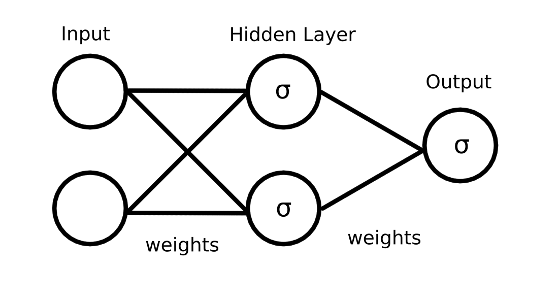
To model the XOR function, we'll be using a simple feedforward neural network with one hidden layer. The network will have two input neurons (one for each input of the XOR function), two hidden neurons, and one output neuron. The architecture of the network is as follows:

The output of each neuron is computed as follows: $$output = \sigma\left(\sum_{i=1}^{n} w_i x_i + b \right) $$ Where $w_i$ are the weights, $x_i$ are the inputs, and $b$ is the bias term. The weights and biases are the parameters that the network will learn during training.

Backpropagation

In order to train a neural network, we need to adjust the weights and biases based on the error between the predicted output and the true output. This is typically done using a method called backpropagation, which involves computing the gradient of the loss function with respect to the weights and biases, and updating them using gradient descent. The loss function measures how well the network is performing, and we will use the L2 Loss, defined as: $$ L = \frac{1}{m} \sum_{i=1}^{m} (y^{(i)} - \hat{y}^{(i)})^2 $$ Where $m$ is the number of training examples, $y^{(i)}$ is the true output for the $i$-th example, and $\hat{y}^{(i)}$ is the predicted output. During backpropagation, we compute the gradients of the loss function with respect to each weight and bias in the network using the chain rule of calculus. This allows us to determine how much each parameter contributes to the overall error. Once we have the gradients, we can update the weights and biases using gradient descent: $$ w_i := w_i - \eta \frac{\partial L}{\partial w_i} $$ $$ b := b - \eta \frac{\partial L}{\partial b} $$ Where $\eta$ is the learning rate, which controls how much we adjust the parameters at each step.

Computing Gradients

In order to compute these gradients, we need to perform a forward pass, which involves computing the outputs of each neuron in the network given the input data. This allows us to compute the loss and then backpropagate the error through the network to compute the gradients. In order to compute the gradients, we'll first define the parameters of the network using the diagram above as a guide:

Input → hidden:

$$ weights: ( W^{(1)} = \begin{bmatrix} w_{11} & w_{12} \\ w_{21} & w_{22} \end{bmatrix} ) $$ $$ biases: ( b^{(1)} = \begin{bmatrix} b_{1} \\ b_{2} \end{bmatrix} ) $$

Hidden → output:

$$ weights: ( W^{(2)} = \begin{bmatrix} v_{1} & v_{2} \end{bmatrix} ) $$ $$ biases: ( b^{(2)} = b_3 ) $$

Forward pass:

$$z^{(1)} = W^{(1)} x + b^{(1)}$$ $$a^{(1)} = \sigma(z^{(1)})$$ $$z^{(2)} = W^{(2)} a^{(1)} + b^{(2)}$$ $$\hat{y} = \sigma(z^{(2)}) $$

Now we compute the output layer gradients. $$\frac{\partial L}{\partial \hat{y}} = \hat{y} - y $$ $$\frac{\partial \hat{y}}{\partial z^{(2)}} = \hat{y}(1 - \hat{y})$$ So, $$ \delta^{(2)} = (\hat{y} - y) \cdot \hat{y}(1 - \hat{y}) $$ Now for the weights and bias:$$ \frac{\partial L}{\partial W^{(2)}} = \delta^{(2)} (a^{(1)})^T$$ $$\frac{\partial L}{\partial b^{(2)}} = \delta^{(2)} $$

Finally, we compute the hidden layer gradients and propagate the error backward. $$ \delta^{(1)} = (W^{(2)})^T \delta^{(2)} \odot a^{(1)} (1 - a^{(1)}) $$ Then: $$ \frac{\partial L}{\partial W^{(1)}} = \delta^{(1)} x^T $$ $$\frac{\partial L}{\partial b^{(1)}} = \delta^{(1)} $$

Training the model

The training process for the XOR dataset involves iterating through each of the 4 training examples some number of times (each pass through the entire dataset is called an epoch). During these iterations, we compute the forward pass to get $ \hat{y} $ for each training example, and use this to compute the loss. We then perform backpropagation to get the gradients and update the weights and biases of the network using gradient descent. We repeat this process for a set number of epochs, or until the loss converges to a satisfactory level. While the XOR function is a simple problem, it serves as a useful example for understanding the basics of neural networks and backpropagation. By training a neural network to learn the XOR function, we can see how the network is able to learn complex, nonlinear relationships in the data through the adjustment of its weights and biases.